Continuing our data manipulation, these further examples can be applied to a cell to extract all kinds of data, and when used together can be particularly powerful when combined with the FIND command. The 4th part will go into detail regarding logic statements 🙂
Finding the nth occurrence of a character with SUBSTITUTE
=FIND(CHAR(1),SUBSTITUTE(<Cell to Check>,”<Character to find>”,CHAR(1),<Occurrence of Character>))
Example:
In the above example the formula references cell A1, looking for the nth occurrence (in this case 3rd) of the character ‘S’. It works by SUBSTITUTE(ing) CHAR(1) for the 3rd occurrence of “S” and returning its position.
I have used this in the past to obtain the nth octet of a MAC address (where that data has not been normalised (i.e. three characters not used for each octet), used in combination with MID discussed in Part 1 – give it a try (clue – you will also need to use LEN discussed in Part 1)!
How do I lookup an object and return related data?
Data lookups:
=VLOOKUP(<lookup value (cell)>, <table to lookup (range)>, <column # containing output data>, <match type>)
vlookup is the most common lookup used within Excel, I tend to use this, and Index/Match (much more powerful) detailed further in this section.
Example:
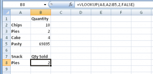
In the above example, the formula in B8 is using A8 as its source. It is looking for ‘Pies’ in the table above (A2:B5) and will return the value in the second column (B). The match type in the above has been set to ‘FALSE’ which means it will return the exact result (rather than a close match if ‘TRUE’ is used).
If the VLOOKUP cannot find what it is looking for in the list, it will return the error #N/A which you will discover will scupper more advance formula. You will need to look at controlling your errors with a little bit of logic; IF statements combined with the use of ISERROR (see part 4).
vlookups great, but I need to obtain data from the left of the lookup?
=INDEX(<Return Value Range>,MATCH(<Lookup value (cell)>,<Lookup Value Range>,0))
Index and match; the old way Excel used to do lookups. Whilst more complex, this complexity adds flexibility by enabling you to perform the likes of (but not limited too) a ‘reverse VLOOKUP’ that’s to say, obtain data from the left!
Example:
Using the same example as vlookup above, but this time with the columns reversed, we are able to return the same valid result :). In cell B8 we have started an index of the range we wish to return, and then matched it against a value we are looking for, in a range this occurs. The “zero” specifies that this is an exact match (rather than “1” – less than, or “-1” greater than).


