PS4 BEEPING AND EJECTING DISC

PS4 Beeping and ejecting disc (or in my case not taking a disc and beeping intermittently all day) – solution:

After suffering this for what seems like an age (with unsuccessful attempts to resolve), and with the pending delivery of Wipeout Omega collection I though again I would trawl the internet for a solution.

Surprisingly I found one that resolved it immediately, simply by turning the manual disc eject screw a few times in the opposite direction for manual ejection (i.e. clockwise).  Follow this support article from Sony:

https://support.us.playstation.com/articles/en_US/KC_Article/PS4-Manually-Eject-a-Stuck-Disc/

More information can be found on the Playstation community here:

http://community.us.playstation.com/t5/Consoles-Peripherals/PS4-Beeping-and-Ejecting-Disc/td-p/43181382/page/2

Update:  It would appear through convection that the shiny removable cover on the PS4 naturally generates static which interferes with the touch buttons.  I have un-clipped this, though still leaving it in place; this has finally cured what appears to be a deisgn flaw!

Share This:

Excel – Data Manipulation (Part 4)

Continuing  our data manipulation, these further examples can be applied to a cell to extract all kinds of data, and when used together can be particularly powerful when combined with the FIND command.

Here have a quick look at the power of logic statements, and again they can be combined with everything we have done previously.

There is much to do with Excel data manipulation, and I have only really scratched the surface, the next series may well look at the various different methods of counting Excel offers, combined with Array formula and a little logic for good measure 🙂


How do I test a value in Excel to see if it meets certain or multiple criteria?

Logic staments:

=IF(text=condition, condition true, condition false)

 To simplify: “If”, “Then”, “Else”.

 Example:
if

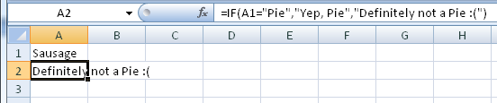
In this example the formula (or logic statement) in A2 is looking for ‘Pie’ in cell A1.  As it is clearly not a pie (rather a tubular food product) THEN (or condition TRUE) is skipped over and ELSE (or condition FALSE) is invoked telling us the contents of A1 is “Definately not a Pie L”.


=OR(condition, condition, condition…)

 Can be used in IF statements as part of a condition, where the answer becomes true if ANY of the conditions met are true.

 Example: or

 In the above example, the IF statement is used along with the OR statement in the initial logic test.  Effectively the combined IF & OR statements check to see if ‘Pies’ OR ‘Peas’ are in cells A1 OR A2 respectively.  IF one or other are then the formula returns ‘There is something you like on the menu’ as is the case here!


=AND(condition, condition, condition…)

Can be used in IF statements as part of a condition, where the answer becomes true if ALL of the conditions met are true.

Example:

and

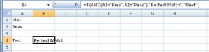
In the above example, the IF statement is used along with the AND statement in the initial logic test.  Effectively the combined IF & AND statements check to see if ‘Pies’ AND ‘Peas’ are in cells A1 AND A2 respectively.  IF they are then the formula returns ‘Perfect match’ as is the case here!


Can I nest IF, OR, AND statements or are they mutually exclusive?

During Christmas cover, I was IM’d asking this very question, the person in question was fairly Excel literate my response was:

=IF(OR(AND(1=x,2=x),AND(3=x,4=x)),THEN,ELSE)

The penny immediately dropped 🙂  Just think logically and carefully about the conditions you are setting out to achieve.  You can nest most if not all Excel formula 🙂


Can I turn an output error from a formula into a meaningful value?

=ISERROR(value)

Yes you can :).  Used primarily as part of a logic statement with a nested IF.  Instead of an error producing a #VALUE error, the error can be specified, for example “” to leave the cell blank.

Example 1 – a formula creating in error:

iserror1

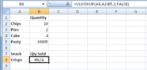
In this example we can see a lookup attempting to return the number of snacks sold, in this case the Value in A8.  Clearly the specified table above has no ‘Crisps’ so the not so useful error code of #N/A is produced.

Example 2 – the use of iserror (in conjunction with a logic statement).

iserror2

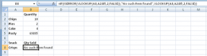
With this example, you can see the previous formula in use along with a logic condition.  In laymen’s terms, IF there IS(an)ERROR doing the LOOKUP then tell me that there is ‘No such Item found’ else do the LOOKUP again, and give me the result.

This way you have more control over your errors, and for example, you can effectively nest IF statements and not be tripped up if part of the formula was to produce an error.  This way, excel is no longer going to produce an uncontrolled error, you are fully in charge.

Share This:

Excel – Data Manipulation (Part 3)

Continuing  our data manipulation, these further examples can be applied to a cell to extract all kinds of data, and when used together can be particularly powerful when combined with the FIND command.  The 4th part will go into detail regarding logic statements 🙂


Finding the nth occurrence of a character with SUBSTITUTE

=FIND(CHAR(1),SUBSTITUTE(<Cell to Check>,”<Character to find>”,CHAR(1),<Occurrence of Character>))

Example:

nthchar

In the above example the formula references cell A1, looking for the nth occurrence (in this case 3rd) of the character ‘S’.  It works by SUBSTITUTE(ing) CHAR(1) for the 3rd occurrence of “S” and returning its position.

I have used this in the past to obtain the nth octet of a MAC address (where that data has not been normalised (i.e. three characters not used for each octet), used in combination with MID discussed in Part 1 – give it a try (clue – you will also need to use LEN discussed in Part 1)!


How do I lookup an object and return related data?

Data lookups:

=VLOOKUP(<lookup value (cell)>, <table to lookup (range)>, <column # containing output data>, <match type>)

vlookup is the most common lookup used within Excel, I tend to use this, and Index/Match (much more powerful) detailed further in this section.

Example:

vlookup

 In the above example, the formula in B8 is using A8 as its source.  It is looking for ‘Pies’ in the table above (A2:B5) and will return the value in the second column (B).  The match type in the above has been set to ‘FALSE’ which means it will return the exact result (rather than a close match if ‘TRUE’ is used).

If the VLOOKUP cannot find what it is looking for in the list, it will return the error #N/A which you will discover will scupper more advance formula.  You will need to look at controlling your errors with a little bit of logic; IF statements combined with the use of ISERROR (see part 4).


vlookups great, but I need to obtain data from the left of the lookup?

=INDEX(<Return Value Range>,MATCH(<Lookup value (cell)>,<Lookup Value Range>,0))

Index and match; the old way Excel used to do lookups.  Whilst more complex, this complexity adds flexibility by enabling you to perform the likes of (but not limited too) a ‘reverse VLOOKUP’ that’s to say, obtain data from the left!

Example:

indexmatch


Using the same example as vlookup above, but this time with the columns reversed, we are able to return the same valid result :).  In cell B8 we have started an index of the range we wish to return, and then matched it against a value we are looking for, in a range this occurs.  The “zero” specifies that this is an exact match (rather than “1” – less than, or “-1” greater than).

Share This:

Excel – Data Manipulation (part 2)

Continuing  our data manipulation, these further examples can be applied to a cell to extract all kinds of data, and when used together can be particularly powerful when combined with the FIND command.  Part 3 (it could even be Part 4) will cover this and more! 🙂


An error is returned on a formula that is using a number extracted from a formula in Excel, why?

=VALUE(text)

When manipulating text using the aforementioned formula, it is common to extract numbers from an alphanumeric cell via manipulation or formula, often with the alphanumeric attribute still intact.  The use of VALUE  then forces any cell referenced to be treated as a number, where as formating the cell will not.

An example is where a formula displays a result and is then referenced by another formula. Second formula may error unless the preceding result is reference through the value statement.


How do I change case from lower to upper case in Excel?

=UPPER(text)

Turns selected text into Upper case.

Example:

upper

A2 contains the example formula; it references A1 as its source. Notice the resulting output is in all upper case.


How do I change case from upper to lower case in Excel?

=LOWER(text)

Turns selected text into Lower case.

Example:

lower

A2 contains the example formula; it references A1 as its source. Notice the resulting output is in all lower case.


How do I combine the contents of multiple cells to make a sentance?

=CONCATENATE(text, text, text…) or the continued use of ‘&’

(Where “text” = cell reference)

Can be used to combine multiple cells of data to form a text string

Example:

conc1

A2 contains the example formula; it references A1, B1, C1 and D1 as its source. To add spaces in this illustration I have added a space character between quotation marks (“ “).

Or:

conc2

Again A2 contains the example formula; it references A1, B1, C1 and D1 as its source. Removing “concatenate” you can combine strings with the example above using & instead.

I will leave you to judge which is your preferred, neater solution.


Share This:

Run any application as a service (using SrvStart)

Every so often I have come across circumastances where I have had to run a windows application as a service.  Some of these applications can be run quite happily and have been designed so, and using SC CREATE from the command prompt is usually adequate.

What if that doesn’t work?  Well, I have found a useful little dibber called SrvStart that enables you to run any application as a service, and here follows short concise guide how to (i’ll also assume you have some tech knowledge on how services work) !

Basically there are three steps after downloading SrvStart from the authors (Nick Rozanski) website, and I will take you through just enough to get you started!

First, copy the contents of the zip file to anywhere in your windows machines Path (for example c:\windows).

Secondly, create an ini file for SvcStart to read, this tells SvcStart what application you wish to run, an example can be found below, again copy this into you Path area.

svrstart

Finally, the third step, run a service as you would normally with SC CREATE from an administrator CMD prompt:

SC CREATE MonitorCTRLSVC DisplayName= “MonitorCTRLSVC” binPath= “srvstart.exe MonitorCTLSVC -c c:\windows\MonitorCTRLSVC.ini” start= auto

If successful, this should have created your windows service!

You can the check functionality via task managers services tab, and if you need to make any further configuration changes use the services console from there

To get this particular application to run as a service I had to create a service account so it could interact with the desktop (it’s a monitor control piece of software by a company called Tecton).

There you have it, three easy steps to get anything running as a service!

UPDATE:

As a member of my team spent some time following a documented set of instructions there is something worth noting….

Whilst 99.99% of windows applications are not case sensitive, it would appear svrstart.exe is.  Please take particular care with the .ini file.  The “startup”, “shutdown” variables are case sensitive and should be written as such in your .ini file 🙂

During this fault finding I found you can also use svrstart to install the service, so the cmd line becomes a little simpler, from the above it would become:

srvstart install MonitorCTRLSVC –c “c:\windows\MonitorCTRLSVC.ini”

Either way the result is exactly the same 🙂

Share This:

Excel – Data Manipulation (part 1)

Particularly useful, these following examples can be applied to a cell to extract all kinds of data, and when used together can be particularly powerful when combined with the FIND command, though a little more on that in another post 🙂


How do I select a certain number of characters in a cell from the left in Excel?

=LEFT(text,[# of Chars])

Takes the characters from Left side of specified cell.

Example:

LEFT

A2 contains the example formula; it references A1 as its source, and take the first 3 characters from the left.


How do I select a certain number of characters in a cell from the right in Excel?

=RIGHT(text,[# of Chars])

Takes the characters from Right side of specified cell.

Example:

Right

A2 contains the example formula; it references A1 as its source, and take the first 3 characters from the left.


 How do I select text from the middle of a cell in Excel?

=MID(text,start #,[# of Chars])

Takes characters from anywhere in a cell, starting at the specified start point).

Example:

mid

A2 contains the example formula; it references A1 as its source. The start # is taken as the P in ‘Pies’ which is 25 characters from the beginning of the cell. The number of characters extracted is 4, giving the output from the sentence as ‘Pies’.


 How can I return the length of text in a cell in Excel?

=LEN(text)

Returns the length of data contained within a cell.

Example:

Len

A2 contains the example formula; it references A1 as its source. It returns the length of the string in A1, in this case 4.

Share This: